WorkoutWednesday 2021: Week 2

This week’s WorkoutWednesday comes to us from Ann Jackson and was very practical, especially for those of us consultants who do any work within the retail space. The challenge was to create a Customer Lifetime Value (CLTV) matrix to show the average value of a customer with each quarter throughout their lifetime. Essentially, it is a way to value the whole future relationship with a customer. On the surface, this was quite straightforward and I utilized a mix of level of detail and table calculations to create the viz. However, the “extra credit”, as Ann put it, was really the icing on the cake and was addressed at the end of this post.

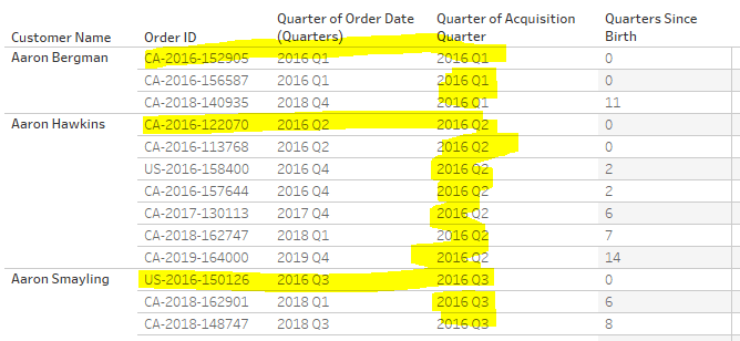
Classify customer by the first quarter they ordered

For every customer, there may be multiple orders over their lifetime. We need to find the date of the first order, and display it as the quarter and year. To calculate this, we can use a level of detail (LOD) calculation:

Acquisition Quarter
{FIXED [Customer Name]: MIN([Order Date (Quarters)])}

This calculation finds the minimum order date (in quarters) for each customer.

Once we have this date, we need to calculate the difference between each order date and this first quarter and report it also in quarters.

Quarters Since Birth
DATEDIFF(‘quarter’,[Acquisition Quarter],[Order Date (Quarters)])

The DATEDIFF function finds the difference between two dates and returns the number based on these noted date interval (in this case quarter).

Now that these initial calculations are created, we can build the shell of the matrix. We start by taking the Acquisition Quarter to Rows and Quarters Since Birth to Columns. As the Acquisition Quarter is a date, we have to decide how to display it. By default, when you bring a date field into the view it defaults to displaying it at the year level. However, we want this to display as the quarter and year. To change the granularity of the date, right click on the date field and select Quarter (where the example shows both the quarter and the year). This will create a continuous date value. We want this to be displayed as discrete values, so we must select discrete from the options.

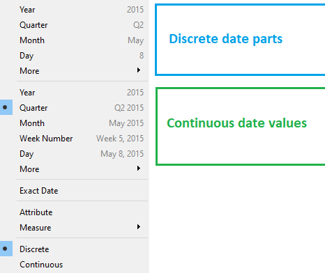
Dates are automatically hierarchies. This means that using the Acquisition Quarter field (a date) will by default allow the user to click through any part of the hierarchy. As we want this to always just be the quarter/year, we can create a custom date calculation (ACQUISITION QUARTER) to create a field that can only be displayed as date value of quarter and use this field on Rows.

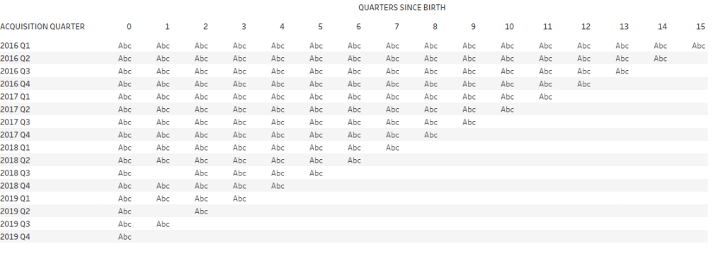
The Abc shows all combinations of Acquisition Quarter and Quarters Since Birth where there is data within the SuperStore data set.

Total Customers per Quarter

We want to determine how many customers first ordered in each of the quarters. Again, we will use a level of detail calculation:

CUSTOMERS
WINDOW_MAX(MAX({FIXED [ACQUISITION QUARTER]:COUNTD([Customer Name])}))

The calculation counts each customer only once for each Acquisition Quarter. We then use the WINDOW_MAX function to return the max of these values, but we want to compute this going across the table. Bring this new field to Rows, set the scope and direction to table across and change the field to discrete so you have the values only and no axis.

Calculate the Customer Lifetime Value (CLTV)

The Customer Value is measured as the Sales per Customer. The Customer Lifetime Value uses a running sum over time (in this case quarters since birth) to determine the lifetime value.

Customer Value

SUM(Sales)
/
[CUSTOMERS]

Taking this one step further, we can modify this field to use the RUNNING_SUM of Sales to calculate the Customer Value field to show the Customer Lifetime Value.

CLTV

RUNNING_SUM(SUM([Sales]))
/
MAX({FIXED [ACQUISITION QUARTER]: COUNTD([Customer Name])})

Be sure to compute the CLTV table calculation as Table Across.

Add a copy of CLTV to filters and show only the non-null values.

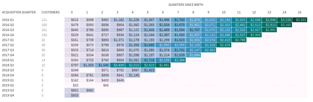
Notice two squares without any data. We will address the potential need for padding the data at the end.

Formatting

Adding Custom Color Palettes

We were provided with the specific color palette to use from Jacob Olsukfa’s great dashboard on Color Palettes for Tableau on Tableau Public. You can customize the color palettes available within Tableau by modifying your preferences.tps file. This file is stored within your My Tableau Repository directory (often within My Documents). From Jacob’s dashboard, you can download the entire preferences file or copy text from the file and add it to your existing preferences.tps.

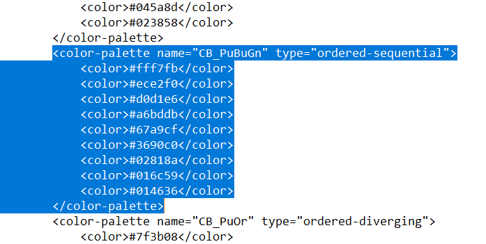
You will need to close and reopen Tableau for the changes to take effect.

Alignment/Borders/White Shading

The columns for ACQUISITION QUARTER and CUSTOMERS are centered. White borders are added around the squares. Additionally, we want to have any cells without any values show up as white. In order to do this, we need to exclude the nulls from the view. Filter the view using CLTV to show the non-null values only.

Tooltips

It is always important to spend some time cleaning up the tooltips with each viz that you create. It helps set apart unfinished views from finished ones, providing that extra bit of polish to a viz. In this case here, we are providing all the details shown in the visual, but also using those values in a sentence to make it easier to understand the customer lifetime value.

<ACQUISITION QUARTER>
CUSTOMER LIFETIME VALUE (CLTV): <Running Sum of AGG(Customer Value)>
TOTAL CUSTOMERS: <AGG(CUSTOMERS)>
QUARTER(S) SINCE BIRTH: <QUARTERS SINCE BIRTH>

After <QUARTERS SINCE BIRTH> quarter(s), customers acquired in <ACQUISITION QUARTER> are worth an average of <Running Sum of AGG(Customer Value)> each.

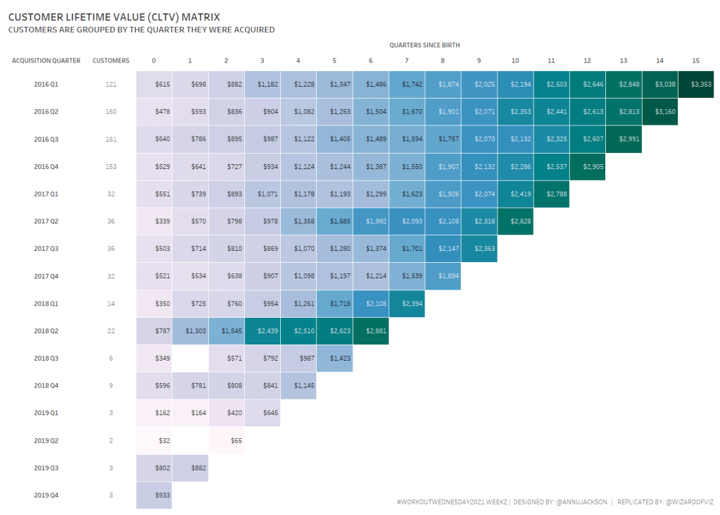
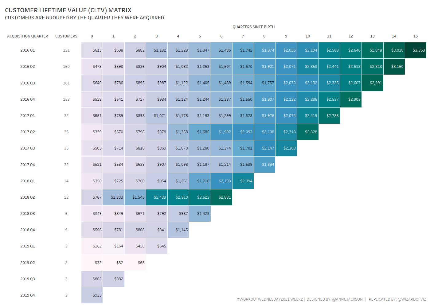
Revisiting the Data Gaps

First it should be mentioned that when you see gaps like those in the view above, you should first ask yourself (and your client) if there is value in the gaps or if instead you want to fill in the data. If we are trying to easily identify those quarters where we did not have repeat business from customers who first ordered in a specific quarter, we may want to keep the viz as is. If, instead, we want to see the customer lifetime value regardless if there were any new sales in a quarter we can adjust our CLTV calculation to handle these null cases.

** I initially started down a different path with this calculation, but admittingly looked at Ann’s solution to see her approach.

CLTV_Padded

IF IFNULL(MAX([QUARTERS SINCE BIRTH]),LOOKUP(MAX([QUARTERS SINCE BIRTH]),-1))
<DATEDIFF(‘quarter’, IFNULL(MAX([ACQUISITION QUARTER]),LOOKUP(MAX([ACQUISITION QUARTER]),-1)) ,#10/01/2019#)
THEN

IFNULL(RUNNING_SUM(SUM([Sales])),LOOKUP(RUNNING_SUM(SUM([Sales])),-1)) /
/
IFNULL(MAX({FIXED [ACQUISITION QUARTER]: COUNTD([Customer Name])}) ,LOOKUP(MAX({FIXED [ACQUISITION QUARTER]: COUNTD([Customer Name])}),-1))

ELSE
RUNNING_SUM(SUM([Sales]))
/
MAX({FIXED [ACQUISITION QUARTER]: COUNTD([Customer Name])})
END

Let’s look at this one step at a time.

First, for instances where we have no value for a given Quarters Since Birth, we want to return the previous Quarters Since Birth.

Next, we want to then check this value and make sure that is less than the difference (in quarters) between the last quarter (with a start date of 10/1/2019) and either the Acquisition Quarter, or if it is null, lookup the previous acquisition quarter.

If the quarters since birth is less than the calculated difference, then if the running sum of sales is null, use the previous running sum of sales and divide it by the calculations for customers unless that value is null, in which case use the previous value.

If there are no null values, simply calculate the CLTV as prior — as the running sum of sales divided by the customers.

Phew! That’s certainly enough to make your head spin. I find it very helpful when I have very complex, multi-step calculation to comment out what each step does. Additionally, I will often work through each part independently to make sure it is doing exactly what I expect and then piece it all back together.

On our view, we can now replace all instances of CLTV with CLTV_Padded. Double check to make sure our scope and direction are set to Table Across.

I thoroughly enjoyed this exercise, and while the basic view was rather simple, the methodology for padding the data would be very useful in similar situations. I look forward to implement one of these charts sooner, rather than later for my retail clients.